>>> sorted([3, 5, 1, 2, 9])[1, 2, 3, 5, 9]Introduction to Software Engineering (CSSE 1001)
A classical problem of computer science is that of sorting a list of items.
This begs a couple questions:
and, if so,
Let us invest five different ways that this problem with two goals in mind:
This topis is part of the transition from software engineering into computer science.
An algorithm is a strategy for solving a problem that can be described independently of Python (or indeed any programming language). Strictly speaking, an algorithm is an ordered set of unambiguous instructions that eventually terminates. Algorithms are an important part of computer science because it is not always obvious how to solve a problem using a computer, and even when we know how, we may not know how to do it quickly.
We turn our focus now on algorithms that sort lists in, say, ascending order. Python has two built-in functions (ones that do not require calling a library) that accomplish this:
>>> sorted([3, 5, 1, 2, 9])[1, 2, 3, 5, 9]and
>>> xs = [3, 5, 1, 2, 9]
>>> xs.sort()
>>> xs
[1, 2, 3, 5, 9]Notice that sorted is a function that given a list returns a new list whereas sort is a method that sorts the list in-place. Generally speaking it is better to sort the list in-place because this requires (at least) half the amount of memory.
We will restrict ourselves to a single list action then use that action to sort the list. The sorting algorithms are named by this action.
def select(xs: list[int]) -> int | None:
    """
    Return the _index_ of the largest element of <xs>.
    """
    current_largest_element = -float('inf')
    current_largest_index = None

    for k, x in enumerate(xs):
        if x > current_largest_element:
            current_largest_element = x
            current_largest_index = k

    return current_largest_index
>>> xs = [5, 2, 9, 10, 3, 2, 4, 8, 1, 3]
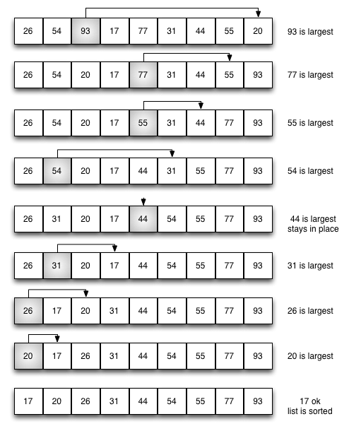
>>> select(xs)3>>> select([1])0>>> select([0, 1, 2])2>>> select([2, 1, 0])0>>> select([1, 2])1As illustrated below, selection sort works by selecting the largest element of the list moving it to the back of the list, while decrementing the index of the back of the list.
And the following function realizes this algorithm.
def selection(xs: list[int]):
    """
    Sort the list <xs> in ascending order _in-place_.
    """

    for k in range(len(xs),0,-1):  # decrement from back of list

        # find largest element in first k elements
        pos_largest_element = select(xs[:k])

        # swap this largest element with the back of the list
        xs[k-1], xs[pos_largest_element] = \
            xs[pos_largest_element], xs[k-1]

    return
>>> xs = [5, 2, 9, 10, 3, 2, 4, 8, 1, 3]
>>> selection(xs)
>>> xs[1, 2, 2, 3, 3, 4, 5, 8, 9, 10]Now, despite the fact we have faithfully sorted a list, our implementation has some issues. When we list slice, as we do when invoking select(xs[:k]), Python will create a new list and pass that new list to select. This means sorting a list of length 100 requires we store \(100 + 99 + \cdots + 2 + 1 = 5050\)
elements (proportional to the square of the original list size). This is not fit for purpose because we may want to sort lists that are so big they totally fill our memory. This is the primary advantage of doing in-place sorts — they are much more spatially efficient, albeit trickier to implement.
We can modify our implementation of selection sort to avoid list-slicing by moving the code for select into selection.
def selection(xs: list[int]) -> list[int]:
    """
    Sort the list <xs> in ascending order _in-place_.
    """

    for j in range(len(xs),0,-1):  # decrement from back of list

        # START SELECT (position of largest element in xs[:j])
        current_largest_element = -float('inf')
        current_largest_index = None

        for k in range(j):
            if xs[k] > current_largest_element:
                current_largest_element = xs[k]
                current_largest_index = k
        # FINISH SELECT

        # swap
        xs[j-1], xs[current_largest_index] = \
            xs[current_largest_index], xs[j-1]

    return
>>> xs = [5, 2, 9, 10, 3, 2, 4, 8, 1, 3]
>>> selection(xs)
>>> xs[1, 2, 2, 3, 3, 4, 5, 8, 9, 10]Now our our function sorts this list without having to duplicate any elements.
def insert(y: int, xs: list[int]) -> list[int]:
"""
Insert <y> into <xs> so that <xs> remains sorted.
Precondition:
<xs> is ascended sorting
"""
for k, x in enumerate(xs):
if y <= x:
return xs[:k] + [y] + xs[k:]
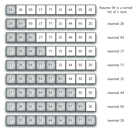
return xs + [y]>>> insert(3, [1, 2, 4])[1, 2, 3, 4]>>> insert(3, [1, 2])[1, 2, 3]>>> insert(0, [1, 2])[0, 1, 2]>>> insert(0, [])[0]To utilize insert to sort a list is fairly trivial. If we want to sort the list xs we simply insert (starting with an empty list which is sorted by definition) every element of xs one at a time. The list we are inserting into will always be left sorted and thereby will always satisfy the precondition for insert.
def insertion(xs: list[int]) -> list[int]:
    """
    Return (a copy of) <xs> but in ascending order.
    """

    ys = []                 # start with empty (sorted) list
    for x in xs:
        ys = insert(x, ys)  # repeatedly insert into
                            # (guaranteed sorted) list
    return ys
>>> xs = [5, 2, 9, 10, 3, 2, 4, 8, 1, 3]
>>> insertion(xs)[1, 2, 2, 3, 3, 4, 5, 8, 9, 10]Astute readers will have noticed that we have again used list slicing in order to implement this particular sorting algorithm. This can be rectified by inserting into the front of the list rather than a new list (as illustrated below).
We omit the in-place insertion algorithm because it is fairly nuanced and distracting from our ultimate goal. These sorting algorithms are covered in much greater detail in COMP3506 (Algorithms & Data Structures).
Bubble sort is among the easiest of the sorting algorithms to implement. We simply look at adjacent elements in the list and swap them when they are out of order. Looking at all adjacent pairs of a list is called a pass and after each pass the largest out-of-place element “bubbles” to the top.
The following illustrates one pass of the list where the element 93 bubbles to the top.
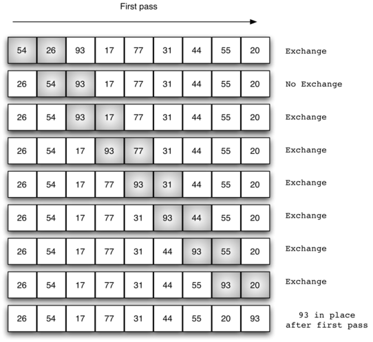
If we make a pass and execute no swaps, then the list must be sorted. The following is an implementation of this idea.
def bubble(xs: list[int]) -> None:
    """
    Sorts the list <xs> in ascending order _in-place_.
    """

    has_swapped = True  # for detecting if swaps occurred
    while has_swapped:
        has_swapped = False
        for k in range(len(xs)-1):
            if xs[k] > xs[k+1]:
                xs[k], xs[k+1] = xs[k+1], xs[k]  # swap
                has_swapped = True

    return None
>>> xs = [5, 2, 9, 10, 3, 2, 4, 8, 1, 3]
>>> bubble(xs)
>>> xs[1, 2, 2, 3, 3, 4, 5, 8, 9, 10]Because we know that after \(n\) bubble-passes of a list, that \(n\) elements (from the back) are necessarily in order, we can improve our implementation by stopping our bubbling when we hit the sorted part of the list. This eliminates the need to tests if swaps are made because eventually the sorted part of the list is the entire list.
def bubble(xs: list[int]) -> list[int]:
    """
    Sorts the list <xs> in ascending order _in-place_.
    """

    if len(xs) < 2:
        return xs

    for j in range(1, len(xs)):  # counts bubble passes
        for k in range(len(xs)-j):  # decrements back of list
            if xs[k] > xs[k+1]:
                xs[k], xs[k+1] = xs[k+1], xs[k]  # swap

    return
>>> xs = [5, 2, 9, 10, 3, 2, 4, 8, 1, 3]
>>> bubble(xs)
>>> xs[1, 2, 2, 3, 3, 4, 5, 8, 9, 10]def merge(xs: list[int], ys: list[int]) -> list[int]:
"""
Return sorted(xs+ys).
Precondition:
<xs> is sorted.
<ys> is sorted.
"""
zs = []
while xs and ys: # at least one list is non-empty
if xs[0] < ys[0]:
zs.append(xs.pop(0))
else:
zs.append(ys.pop(0))
# xs or ys may still have elements left
zs.extend(xs)
zs.extend(ys)
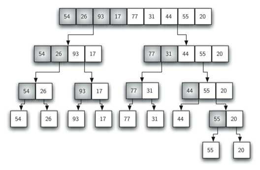
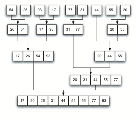
return zs>>> merge([1, 3, 5], [2, 4])[1, 2, 3, 4, 5]>>> merge([1], [2])[1, 2]>>> merge([1], [])[1]>>> merge([], [2])[2]>>> merge([], [])[]This is the first recursion sorting algorithm we consider. To sort a list with merge we cut the list in half and sort (recursively) the halves and then merge the outcome. Lists of length zero or one are sorted by definition and constitute the smallest sorting problem (the base case). This process is illustrated below.
def merge_sort(xs: list[int]) -> list[int]:
    """
    Return (a copy of) <xs> but in ascending order.
    """

    # base case
    if len(xs) < 2:
        return xs

    # cut list in two pieces
    n = len(xs)
    ys, zs = xs[:n//2], xs[n//2:]

    return merge(merge_sort(ys), merge_sort(zs))
>>> xs = [5, 2, 9, 10, 3, 2, 4, 8, 1, 3]
>>> merge_sort(xs)[1, 2, 2, 3, 3, 4, 5, 8, 9, 10]Merge-sort can (and should) also be made in-place (but we omit this).
This is another recursive sorting algorithm that works like merge sort in that we sort the list by breaking it into smaller pieces which are recursively sorted. Two groups are formed by choosing a pivot and collecting those elements less than (or equal to) the pivot into a “left” group and those not into a “right” group. We know the (sorted) list of left-elements are all less than the (sorted) list of right-elements and therefore we can just append them while making sure to place the pivot itself in the middle. The resulting list is sorted.
Choosing a clever pivot can make quick-sort very fast, but for our purposes we simply choose the head of the list as our pivot.
def quick_sort(xs: list[int]) -> list[int]:
    """
    Return (a copy of) <xs> but in ascending order.
    """

    if len(xs) < 2:
        return xs

    pivot, tail = xs[0], xs[1:]

    left = [x for x in tail if x <= pivot]
    right = [x for x in tail if x > pivot]

    return quick_sort(left) + [pivot] + quick_sort(right)
>>> quick_sort([5, 2, 9, 10, 3, 2, 4, 8, 1, 3])[1, 2, 2, 3, 3, 4, 5, 8, 9, 10]Quick-sort can (and should) also be made in-place (but we omit this).
We have written five functions that all accomplish the same task faithfully.
Which one is best?
To see if there is even any difference we can run some experiments by timing how long each method takes to sort random lists of various sizes. To be fair let us have each method sort 50 random list and average the times.
import random
import timeit

def random_list(n: int) -> list[int]:
    """
    Return a random list of length-<n> of integers in range(1000)
    """
    return [random.randint(0,1000) for _ in range(n)]

def experiment(n: int):
    """
    Print the average number of seconds required of each algorithm to
    sort a random list of <n> integers in range(1000)
    """

    print(f"Sorting size |xs| = {n}")

    for algorithm in [selection, insertion, bubble, merge_sort, quick_sort]:
        time = 0
        for _ in range(10):
            xs = random_list(n)
            time += timeit.timeit(lambda: algorithm(xs), number=1)

        # we are using fancy print formatting here
        print(f"{algorithm.__name__:>11}  \t {time/10:>5.3f}s")
>>> experiment(10**3)Sorting size |xs| = 1000
selection 0.007s
insertion 0.005s
bubble 0.020s
merge_sort 0.001s
quick_sort 0.001s>>> experiment(10**4)Sorting size |xs| = 10000
selection 0.731s
insertion 0.704s
bubble 2.112s
merge_sort 0.014s
quick_sort 0.009s>>> experiment(10**5)Sorting size |xs| = 100000
selection 74.872s
insertion 74.866s
bubble 214.060s
merge_sort 0.732s
quick_sort 0.237sSo, clearly, some the sorting algorithms are better than others.
We summarize the timing results of the previous section in the following table.
| Algorithm | \(n=10^3\) | \(n=10^4\) | \(n=10^5\) |
|---|---|---|---|
| Selection | 0.007s | 0.731s | 74.87s |
| Insertion | 0.005s | 0.704s | 74.87s |
| Bubble | 0.020s | 2.122s | 214.1s |
| Merge | 0.001s | 0.014s | 0.732s |
| Quick | 0.001s | 0.009s | 0.237s |
Notice that for selection, insertion, and bubble a ten-fold increase in list size corresponds to a hundred-fold increase in processing time. Whereas for merge and quick sort, the increase in processing time is just a tad more than ten-fold.
It is this relationship between input size and run-time that we are interested in more-so than the raw timings because they enable us to extrapolate wait times of larger inputs from smaller inputs, giving us some expectation of how long a function will take to execute before we run it. In computer science this is called the algorithm’s complexity.
We measure the complexity of an algorithm by bounding the number of relevant operations it performs rather than giving a precise accounting of operations (which is only possible for a given input). Our sorting algorithms are dominated by comparisons and swaps so this is what we will count. Let us start with selection.
def selection(xs: list[int]) -> list[int]:

    # let n = len(xs)

    for j in range(len(xs),0,-1): # repeats n many times

        current_largest_element = -float('inf')
        current_largest_index = None

        for k in range(j): # repeats (at most) n many times,
                           # n many times = n**2 many times
            if xs[k] > current_largest_element:  # (at most) n**2 many comparisons
                current_largest_element = xs[k]
                current_largest_index = k

        # n many swaps
        xs[j-1], xs[current_largest_index] = \
            xs[current_largest_index], xs[j-1]

    return

# The number of swaps and comparisons (at most) n**2 + n
So the number of swaps and comparisons that selection does is (at most) \(n^2 + n\). However when \(n\) becomes large this measurement becomes totally dominated by \(n^2\). Because of this, we say the complexity of selection sort is \(\mathcal{O}(n^2)\) rather than report the more precise count.
This aligns with our experiments. We have determined it takes about \(n^2\) many operations to selection sort a list of length \(n\). Therefore to sort a list of length \(10 n\) requires \((10n)^2 = 100 n^2\) operations — a one-hundred-times increase in cost.
A similar analysis can be done on insertion and bubble to determine their complexities are also \(\mathcal{O}(n^2)\). Even though bubble runs way slower we consider it to as good/bad as the other two in its complexity analysis.
To determine the complexity of merge and quicksort is trickier and requires the Master Theorem which is a result characterizing the complexity of recursive functions. Using that the complexities of both of these algorithms can be determined to be \(\mathcal{O}(n \log n)\).
The following is the precise definition of complexity. It looks complicated, but it is merely says a function \(f(n)\) is in the complexity class \(\mathcal{O}(g(n))\) when eventually \(g(n)\) is always larger than \(f(n)\) (up to scaling \(g(n)\)). This is necessary because it takes some time for dominant terms to take over. Consider that \(n\) is actually larger than \(n^2\) on the interval \((0, 1)\).
Definition 1 (Big-Oh Complexity) We say that \(f(n)\) is big-oh of \(g(n)\) and write \(f(n) = \mathcal{O}(g(n))\) when \[ \exists\, c,\, k \in \mathbb{R}^{>0} : \forall n \geq k;\, 0 \leq f(n) \leq cg(n). \] That is, when there is some positive constant \(c\) such that \(f\) is eventually larger than \(cg\).
Example 1 The function \(2x^2 + x + 1 = \mathcal{O}(n^2)\) because for \(x>2\) \[2x^2 + x + 1 < 3x^2.\]
Example 2 The function \(x^3 -\sin(x) = \mathcal{O}(n^3)\) because for \(x>1\) \[x^3 - \sin(x) \leq x^3 + 1 < 2x^3.\]
We will now just give some examples of functions of various complexities. At this introductory level, we are effectively just accounting for embedded loops. Namely, loops in loops will have a multiplicative effect on the complexity whereas loops after loops will have an additive effect.
Any function that is bounded by a fixed number of operations is part of the constant complexity class. This can sometimes be confusing because a function that has loops (even embedded ones) can fall into this class if the loops are not dependent on the input.
Here are some examples of functions in the constant complexity class.
def foo(x: int):
    x += 1   # 1 assignment / addition
             # -----------------------
             # 1 = O(1)
def bar(n: int):
while i < 10**10: # 10**10 comparisons
index += 1 # 10**10 assignments / additions
# ------------------------------
# 2*10**10 = O(1)Here is an example of a function in the linear complexity class.
def spam(n: int):
                       # Number of ops
    while index < n:   # n  comparisons
        index += 1     # n  assignments / additions
                       # --------------------------
                       # 2n + 2 = O(n) operations
Generally speaking, and loop (while or for) that is effected by the size of the input will contribute a \(n\) (linear term) to the complexity.
Here is an example of a function in the quadratic complexity class.
def eggs(n: int):
    while i < n:       # n comparisons
        j = 0          # n assignment
        while j < n:   # n * n comparisons
            j += 1     # n * n assignments / additions
        i += 1         # n assignments / additions
                       # -----------------------------
                       # 2n**2 + 3n = O(n**2)
def ham(n: int):
for _ in range(n): # n increments
for _ in range(n//2): # n * n//2 increments
pass # n * n//2 empty instructions
# ---------------------------
# n**2//2 + n = O(n**2)Notice the multiplicative effect that embedding loops has. Generally speaking embedded loops that both have size proportional to the input will contribute a \(n^2\) (quadratic term) to the complexity.
On the other hand, if the loops are sequenced then the effect is additive.
def green(n: int):
    for _ in range(n):     # n increments
        pass               # n empty instructions

    for _ in range(2*n):   # 2*n increments
        pass               # 2*n empty instructions
                           # ----------------------
                           # 2*n + 4*n = O(n)
Also be careful to ensure the loop is actually proportional to the input, otherwise the contribution is constant. That is, just because a function has embedded loops does not necessary imply the presence of a quadratic term.
def sam(n: int):
    for _ in range(n):         # n increments
        for _ in range(100):   # n*100 increments
            pass               # n*100 empty instructions
                               # ------------------------
# 201*n = O(n)For every embedded loop that is proportional to the input the complexity class will increase from quadratic to cubic and beyond.
def iam(n: int):
    for _ in range(n):           # n increments
        for _ in range(n):       # n*n increments
            for _ in range(n):   # n*n*n increments
                pass             # n*n*n empty instructions
                                 # ------------------------
                                 # 2n**3 + 2n**2 + n = O(n**3)
Logarithmic is an important complexity class because they characterize functions that utilize divide and conquer methods (like merge and quicksort). A list of size \(n\) can be broken in half \(\log_2(n)\) many times and therefore mere_sort will make \(\log_2(n)\) many calls to merge that itself has complexity \(O(n)\).
def merge(xs: list[int], ys: list[int]) -> list[int]:
                                   # let n = len(xs) + len(ys)
    zs = []
    while xs and ys:               # at most n many iterations
        if xs[0] < ys[0]:          # at most n many comparisons
            zs.append(xs.pop(0))   # at most n many appends
        else:
            zs.append(ys.pop(0))   # at most n many appends

    # xs or ys may still have elements left
    zs.extend(xs)                  # at most n many appends
    zs.extend(ys)                  # at most n many appends

    return zs                      # ------------------------
                                   # 6n = O(n)
def merge_sort(xs: list[int]) -> list[int]:
# base case
if len(xs) < 2:
return xs
# cut list in two pieces
n = len(xs)
ys, zs = xs[:n//2], xs[n//2:]
return merge(merge_sort(ys), merge_sort(zs))
# ^ at most log[2](n) many calls to merge which has cost O(n)
# where n = len(xs)Consequently, the complexity of merge_sort is \(\mathcal{O}(n \log n)\). Logarithmic complexities are among the best we can hope as a logs increase exceedingly slowly. This means algorithms with logarithmic complexities are typically fast, as we saw in our experiments.